Expectation of a continuous random variable

Let \(X\) be a discrete random variable taking real values. The expectation of \(X\) is defined by:

\[ \mathbf{E}[X] = \int_{-\infty}^{+\infty} xp(x), \]

where \(p(x)\) is the PDF of \(X\).

Example: The expectation of a uniform random variable

Take a uniform random variable:

\[ X \sim U([a, b]). \]

Its expectation is:

\[\begin{split} \begin{split} \mathbf{E}[X] &= \int_{-\infty}^{+\infty} x p(x) dx\\ &= \int_a^b x \frac{1}{b-a}dx,\;\text{(PDF is zero outside the interval)}\\ &= \frac{1}{b-a}\frac{x^2}{2}|_a^b\\ &= \frac{1}{b-a}\frac{b^2 - a^2}{2}\\ &= \frac{1}{b-a}\frac{(b-a)(b+a)}{2}\\ &= \frac{a+b}{2}, \end{split} \end{split}\]

which makes a lot of sense because it is the point between \(a\) and \(b\).

Interpretation of the expectation of continuous random variables

Mathematically, the expectation is the x-coordinate of the centroid of the area between the x-axis and the PDF, see Fig. 9.

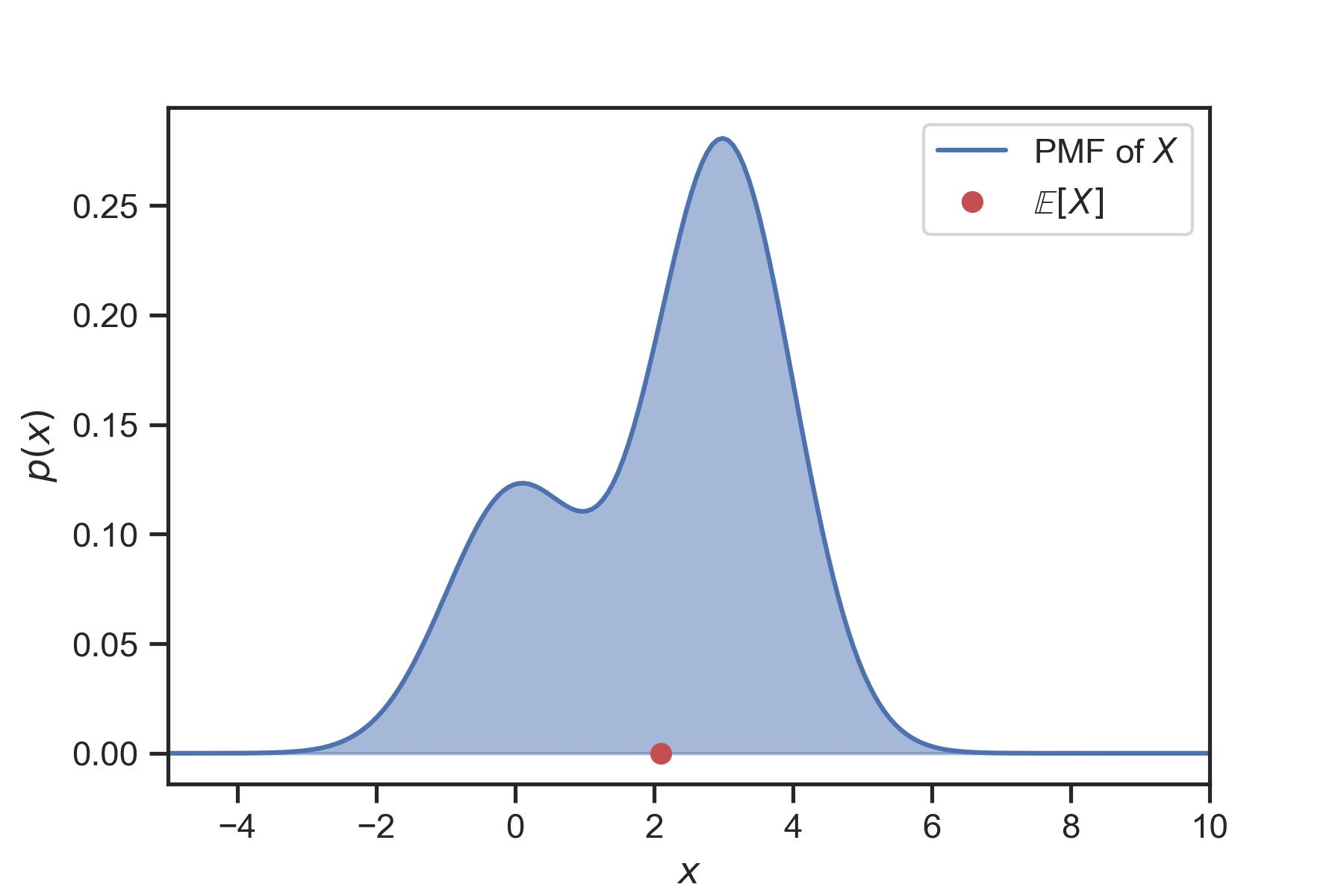
Fig. 9 The expectation of a random variable is the x-coordinate of the centroid of the area between the x-axis and the PDF.

As in the discrete case, you can think of the expectation as the value one should “expect” to get. But, again, take this interpretation with a grain of salt… See Fig. 10 for an example where the expectation is a very improbable value.

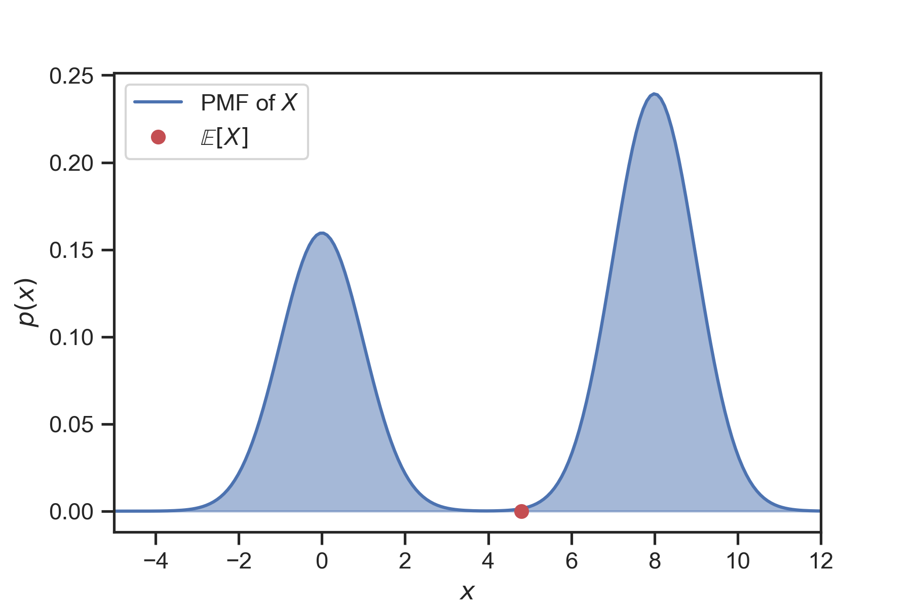
Fig. 10 The expectation of a random variable does not have to be on a high probability region.

Note

In Fig. 10, the PDF of the random variable has two distinct peaks. Each peak of the PDF is called a mode. “Nice” PDF’s have a single mode. They are called unimodal. For unimodal PDF’s the interpretation that the expectation is the value you should expect to get makes a lot of sense. However, a PDF may be multi-modal. Then the expectation is not very useful…