The probability density function¶

The probability

Take a continuous random variable \(X\). The probability density function (PDF) \(f_X(x)\) gives you the probability per unit of \(x\) that \(X\) is in a very small region around \(x\). Intuitively, the definition is:

\[ f_X(x) \approx \frac{p(x < X \le x + \Delta x)}{\Delta x}, \]

for \(\Delta x\) very very small. In other words, \(f_X(x)\) is the probability that \(X\) is between \(x\) and \(x + \Delta x\) divided by \(\Delta x\). It is exactly because you divide by \(\Delta x\) that this is a probability density and not just a probability.

As you have already realized, I do not like writing \(f_X(x)\). So, if there is no ambiguity, I will write instead:

\[ p(x) \equiv f_X(x). \]

Note

Again, this is not the precise mathematical definition of the PDF of a random variable, but it is good enough for our purposes.

There are some properties that the PDF satisfies which you absolutely need to remember. We visualize the most important properties in Fig. 8.

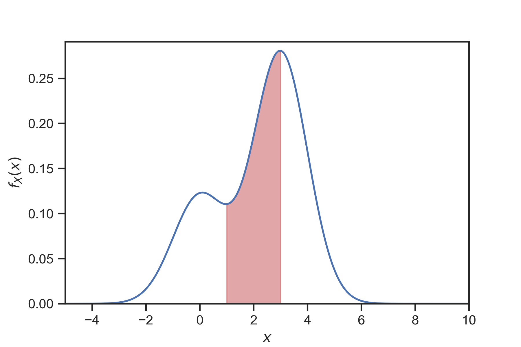
Fig. 8 The PDF of a typical continuous random variable looks like this. It is a non-negative function. The area between the function and the x-axis is one. The probability of the random variable being within a given interval is given by the integral of the PDF over that integral. In this figure \(p(1 < X \le 3) = \int_1^3 p(x)dx\) is the shaded area.¶

PDF Property 1: The PDF is non-negative¶

Because \(p(x)\) is a probability density and probabilities are non-negative, we get that:

\[ p(x) \ge 0. \]

The set of \(x\)’s for which \(p(x)\) is strictly positive is known as the support of the PDF. Obviously, a random variable cannot take any values outside its support.

PDF Property 2: The PDF is the derivative of the CDF¶

Let \(F(x)\) be the CDF of \(X\), see The cumulative distribution function. Then we have:

\[ p(x) = \frac{dF(x)}{dx}. \]

This is interesting! Before proving it, let’s check the units. \(F(x)\) has units of probability. If we divide by \(dx\) we get probability density. This looks promising. Let’s do the proof.

We have:

\[\begin{split} \begin{split} p(x) \approx& \frac{p(x < X \le x + \Delta x)}{\Delta x}\;\text{(definition)}\\ &= \frac{F(x + \Delta x) - F(x)}{\Delta x}\;\text{(CDF Property 4)}. \end{split} \end{split}\]

Now the result follows by taking the limit \(\Delta x\rightarrow 0\).

As a sanity check, let’s look back at Example: Uncertainties in steel ball manufacturing. Does the property hold for what we found there? Our CDF was:

\[\begin{split} F(x) = \begin{cases} 0,&\;\text{if}\;x<0.95\;\text{mm},\\ 10\;\text{mm}^{-1}\cdot (x-0.95\;\text{mm}),&\;\text{if}\;0.95\;\text{mm}\le x\;1.05\;\text{mm},\\ 1,&\;\text{otherwise}. \end{cases} \end{split}\]

Taking the derivative with respect to \(x\) yields:

\[\begin{split} p(x) = \begin{cases} 0,&\;\text{if}\;x<0.95\;\text{mm},\\ 10\;\text{mm}^{-1},&\;\text{if}\;0.95\;\text{mm}\le x\;1.05\;\text{mm},\\ 0,&\;\text{otherwise}, \end{cases} \end{split}\]

which agrees with the constant density we found in our example.

PDF Property 3: The CDF is the integral of the PDF¶

We have:

\[ F(x) = \int_{-\infty}^x p(\tilde{x})d\tilde{x}. \]

This follows directly from PDF Property 2 if we employ the fundamental theorem of calculus.

PDF Property 4: Probability the random variable takes values in a set is the integral of the PDF over the set¶

The probability that \(X\) takes values between \(a\) and \(b\) for \(a<b\) is given by:

\[ p(a < X \le b) = \int_a^b p(x) dx. \]

See Fig. 8 for a visualization. The probability is the area between the PDF, the x-axis, and the endpoints of the interval \([a, b]\).

This is obviously extremely useful because if you have the PDF it allows you to easily calculate probabilities by doing integrals! Let’s prove it:

\[\begin{split} \begin{split} p(a < X \le b) &= F(b) - F(a)\;\text{(CDF Property 4)}\\ &= \int_a^b \frac{dF(x)}{dx} dx\;\text{(fundamental theorem of calculus)}\\ &= \int_a^b p(x)dx\;\text{(PDF Property 2)}. \end{split} \end{split}\]

This property can be generalize. If \(A\) is any set of possible values of \(X\), then:

\[ p(X\in A) = \int_A p(x)dx. \]

PDF Property 5: The PDF integrates to one¶

The property is:

\[ \int_{-\infty}^{+\infty}p(x) dx = 1. \]

In words, the total area between the PDF curve and the x-axis is one. Proving this property is obvious. You just have to notice that:

\[ \int_{-\infty}^{+\infty}p(x) dx = p(-\infty < X \le + \infty) = 1, \]

because \(X\) must take some value.

Note

It is a very common mistake to think that the PDF has to be smaller than one. But the PDF is a probability density not a probability. So, it can take values greater than one. In Example: Uncertainties in steel ball manufacturing the probability density was 10 \(\text{mm}^{-1}\).

Questions¶

You have a random variable \(X\) that measures the mass of an object. What are the units of its PDF \(p(x)\)?

\(\text{kg}^{-1}\) (Correct answer)
\(\text{kg}\)
The PDF does not have units.

Introduction to Data Science for Mechanical Engineers (Lecture Book)

The probability density function

Contents