.md .pdf

Logistic regression

Imagine that you have a bunch of observations consisting of inputs/features \(\mathbf{x}_{1:N}=(\mathbf{x}_1,\dots,\mathbf{x}_N)\) and the corresponding targets \(y_{1:N}=(y_1,\dots,y_N)\). Remember that we say that we have a classification problem when the targets are discrete labels. In particular, if the labels are two, say 0 or 1, then we say that we have a binary classification problem.

The logistic regression model is one of the simplest ways to solve the binary classification problem. It goes as follows. You model the probability that \(y=1\) conditioned on having \(\mathbf{x}\) by:

\[ p(y=1|\mathbf{x},\mathbf{w}) = \operatorname{sigm}\left(\sum_{j=1}^Mw_j\phi_j(\mathbf{x})\right) = \operatorname{sigm}\left(\mathbf{w}^T\boldsymbol{\phi}(\mathbf{x})\right), \]

where \(\operatorname{sigm}\) is the sigmoid function, the \(\phi_j(\mathbf{x})\) are \(m\) basis functions/features,

\[ \boldsymbol{\phi}(\mathbf{x}) = \left(\phi_1(\mathbf{x}),\dots,\phi_M(\mathbf{x})\right) \]

and the \(w_j\)’s are \(m\) weights that we need to learn from the data. The sigmoid function is defined by:

\[ \operatorname{sigm}(z) = \frac{1}{1+e^{-z}}, \]

and all it does is it takes a real number and maps it to \([0,1]\) so that it can represent a probability, see Fig. 12. In other words, logistic regression is just a generalized linear model passed through the sigmoid function so that it is mapped to \([0,1]\).

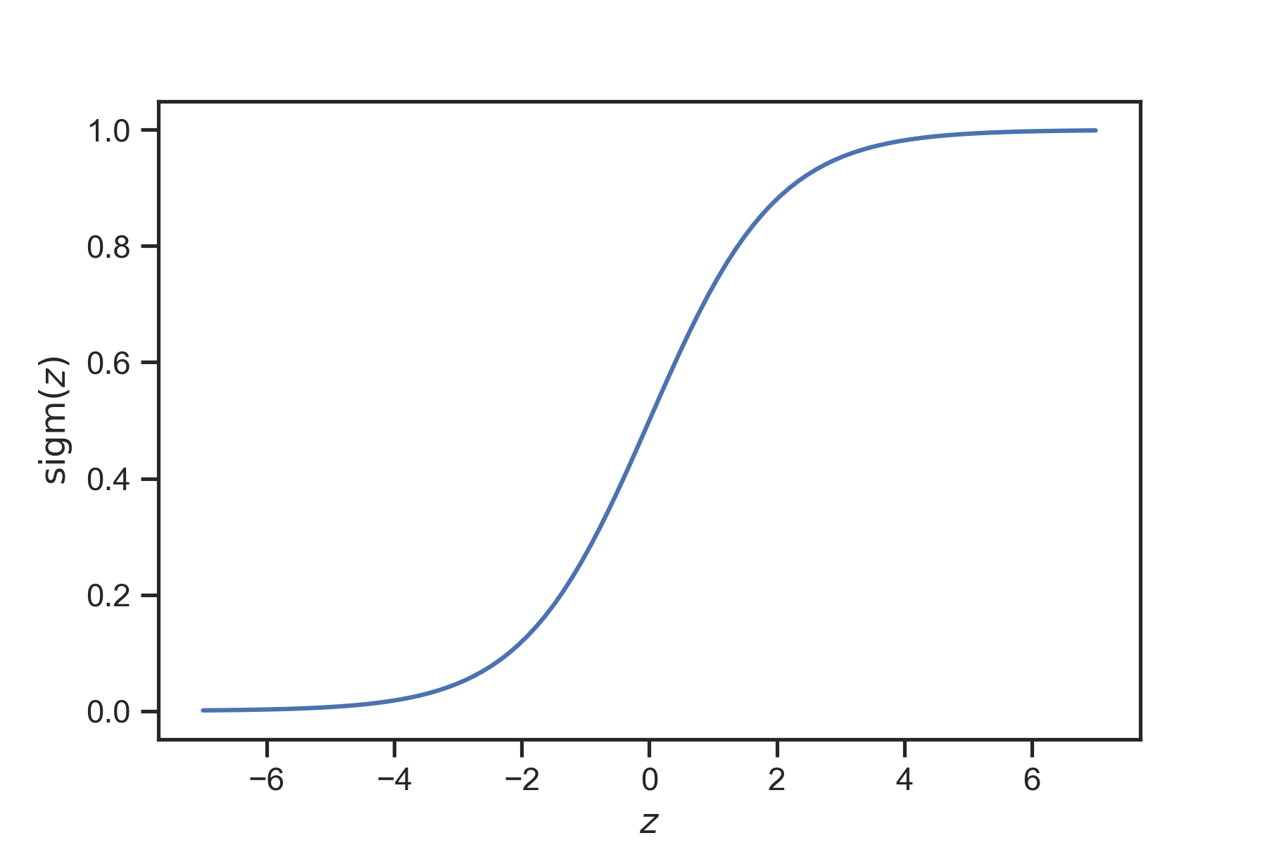
Fig. 12 The sigmoid function takes any number and maps it to the unit interval \([0, 1]\). We use it at the end of models that are supposed to spit out probabilities.

If you need the probability of \(y=0\), it is given by the obvious rule:

\[ p(y=0|\mathbf{x},\mathbf{w}) = 1 - p(y=1|\mathbf{x},\mathbf{w}) = 1 - \operatorname{sigm}\left(\mathbf{w}^T\boldsymbol{\phi}(\mathbf{x})\right) \]

You can represent the probability of an arbitrary label \(y\) conditioned on \(\mathbf{x}\) using this simple trick:

\[ p(y|\mathbf{x},\mathbf{w}) = \left[\operatorname{sigm}\left(\mathbf{w}^T\boldsymbol{\phi}(\mathbf{x})\right)\right]^y \left[1-\operatorname{sigm}\left(\mathbf{w}^T\boldsymbol{\phi}(\mathbf{x})\right)\right]^{1-y}. \]

Notice that when \(y=1\), the exponent of the second term becomes zero and thus the term becomes one. Similarly, when \(y=0\), the exponent of the first tierm becomes zero and thus the term becomes one. This gives the right probability for each case.

The likelihood of all the observed data is:

\[ p(y_{1:N}|\mathbf{x}_{1:n},\mathbf{w}) = \prod_{i=1}^Np(y_i |\mathbf{x}_i, \mathbf{w}) = \prod_{i=1}^N \left[\operatorname{sigm}\left(\mathbf{w}^T\boldsymbol{\phi}(\mathbf{x}_i)\right)\right]^{y_i} \left[1-\operatorname{sigm}\left(\mathbf{w}^T\boldsymbol{\phi}(\mathbf{x}_i)\right)\right]^{1-y_i}. \]

We can now find the best weight vector \(\mathbf{w}\) using the maximum likelihood principle. We need to solve the optimization problem:

\[ \max_{\mathbf{w}}\log p(y_{1:N}|\mathbf{x}_{1:n},\mathbf{w}) = \max_{\mathbf{w}}\sum_{i=1}^N\left\{y_i\operatorname{sigm}\left(\mathbf{w}^T\boldsymbol{\phi}(\mathbf{x}_i)\right)+(1-y_i)\left[1-\operatorname{sigm}\left(\mathbf{w}^T\boldsymbol{\phi}(\mathbf{x}_i)\right)\right]\right\}. \]

Notice that the following maximization problem is equivalent to minimizing this loss function:

\[ L(\mathbf{w}) = -\sum_{i=1}^N\left\{y_i\operatorname{sigm}\left(\mathbf{w}^T\boldsymbol{\phi}(\mathbf{x}_i)\right)+(1-y_i)\left[1-\operatorname{sigm}\left(\mathbf{w}^T\boldsymbol{\phi}(\mathbf{x}_i)\right)\right]\right\}. \]

This is known as the cross-entropy loss function and you are very likely to encounter it if you dive deeper into modern data science. For example, we use the same loss function to train state-of-the-art deep neural networks that classify images. You now know that it does not come out of the blue. It comes from the maximum likelihood principle.

Note

It is not possible to analytically minimize the cross-entropy loss function. The optimization is usually done with a numerical optimization technique. For small datasets, we can use a gradient-based optimization (e.g., the conjugate gradient method, or the Newton-Raphson method). The details of this optimization algorithm are beyond the scope of the present course. You can learn about them in a course like ME 581. For large datasets, this is typically the case for deep learning, we use variants of stochastic gradient descent. To learn more about this take a course like ME 539.

previous

Lecture 16: Classification via logistic regression

next

Example: Logistic regression with one variable (High melting explosives)